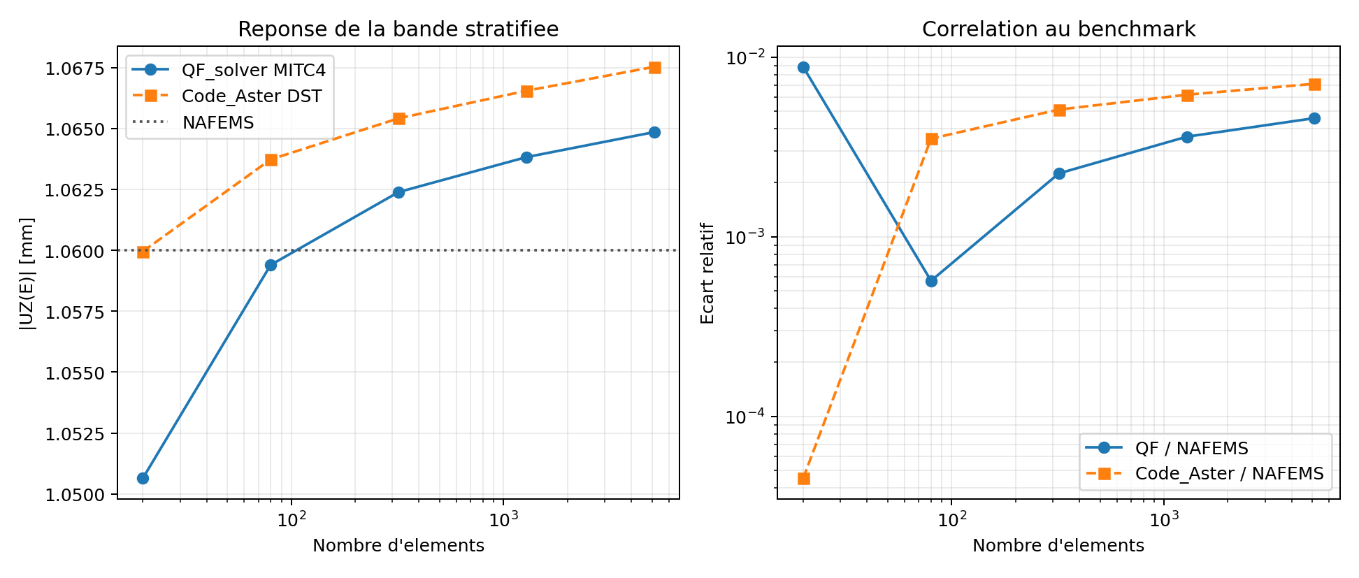
Layer stiffnesses are integrated through thickness into extensional, coupling, and bending matrices.
01 Model and scope
Classical laminate theory represents a perfectly bonded stack of linear orthotropic plies by integrating each rotated plane-stress stiffness through thickness. The three thickness moments produce A (extension), B (extension–bending coupling), and D (bending). This constitutive result is not, by itself, a shell element or a delamination model.
Route assumptions and calculation checks
- Each ply plane-stress stiffness is rotated to shell axes and integrated over its own z interval to form A, B, and D.
- A mirrored material/thickness stack makes the zQ̄(z) integral cancel and B=0; unsymmetric stacks generally couple membrane strain and curvature.
- Ply stresses are recovered at lower/middle/upper positions. MITC4 also adds transverse shear; the current accepted static scope is bounded to selected planar regular meshes.
Useful foundations and prerequisites
02 Essential equations and symbols
Definitions and conventions
- Ply k's plane-stress stiffness transformed from its 1–2 material axes to shell axes.
- Bottom and top coordinates of ply k measured from the laminate mid-plane.
- A, B, D
- 3×3 extensional, extension–bending coupling, and bending stiffness matrices.
- Mid-plane engineering strain and curvature vectors in the declared shell convention.
- N, M
- Membrane force and bending moment resultants per unit width.
- Aₛ
- Separate transverse-shear stiffness used by the Reissner–Mindlin MITC4 shell route.
03 Step by step derivation
Follow the assumptions, equations and discrete operations in order. The full explanation stays visible.
The site separates the ply law, stacking sequence, ABD integration, MITC4 shell kinematics, transverse shear, and failure indicators. The current QF Solver MITC4 laminate implementation adds a shear matrix and weak drilling term beyond ABD; its documented status is bounded and route-specific.
1 · State the laminate kinematic assumptions
The classical laminate law assumes thin, perfectly bonded plies, linear in-plane response, plane stress in each lamina, and a prescribed stacking sequence. In the first-order kinematic model, in-plane strain varies linearly through thickness. Inter-ply displacement jumps and interface opening are not represented.
The sign of curvature depends on the local shell axes and convention. Keep that convention consistent in the input, force resultants, moment resultants, and recovered stresses.
2 · Build each lamina's plane-stress stiffness
Within each ply, axes 1 and 2 follow the material directions in the lamina plane. Elastic reciprocity gives ν21=ν12E2/E1. The reduced stiffness Q maps in-plane engineering strain to in-plane stress; it is not the full 3D orthotropic solid matrix from the preceding card.
The ply angle rotates this law into the shell axes to produce Q̄ₖ. The code performs tensor rotations and converts engineering shear explicitly.
3 · Integrate transformed ply stiffness across thickness
For ply k, Q̄ₖ is constant between interfaces zₖ₋₁ and zₖ. Integrating Q̄ₖ, zQ̄ₖ, and z²Q̄ₖ gives the three classical laminate matrices. A and D are always assembled from every ply; B changes sign with the location of each ply relative to the mid-plane.
With Q̄ in Pa and z in metres, A has units N/m, B has units N, and D has units N·m. N and M are resultants per unit width.
4 · Interpret coupling and a symmetric stack
An unsymmetric sequence generally has B≠0, so a pure membrane resultant can induce curvature and a pure moment can induce mid-plane strain. If the material stiffness distribution is mirrored about z=0, the integrand zQ̄(z) is odd and B vanishes. A balanced layup addresses different in-plane normal/shear coupling terms; it does not automatically imply B=0.
Symmetry is about the complete material-and-thickness sequence, not merely whether angle labels look repeated. Equal ply thickness and mirrored ply properties/orientations are needed for the cancellation.
5 · Recover strains and stresses ply by ply
After solving for ε⁰ and κ, evaluate the strain at each ply's lower face, mid-plane, and upper face. Rotate strain into the ply material axes and use Q for material-axis stress. At an interface, the strains may be kinematically continuous while stresses jump because neighboring plies have different stiffnesses.
Retain both one-sided stresses at interfaces. Averaging across an interface can hide the discontinuity that drives ply-level failure checks.
6 · Connect ABD to the actual MITC4 shell route
The MITC4 shell adds Reissner–Mindlin transverse shear to the in-plane ABD response. QF Solver integrates rotated G13/G23 through the thickness and applies a default shear factor 5/6; membrane–bending cross terms are retained for unsymmetric stacks. A weak drilling stiffness is also used. These additions belong to the shell element route, not to the bare ABD equations.
The v0.2.11 documentation bounds current laminate static evidence to selected planar regular meshes. Distorted/oblique probes remain outside that accepted subset; dynamics, damage evolution, delamination, and industrial decision validation are not implied.
04 Algorithm and implementation
Source excerpt · v0.2.11
The source integrates each rotated ply stiffness over its actual interface interval; the power of z selects A, B, or D.
Functions shown: _integrated_matrix
def _integrated_matrix(self, *, power: int, factor: float) -> np.ndarray:
    interfaces = self.interfaces
    matrix = np.zeros((3, 3), dtype=float)
    for index, ply in enumerate(self.plies):
        lower = interfaces[index]
        upper = interfaces[index + 1]
        matrix += factor * ply.transformed_stiffness * (upper**power - lower**power)
    return 0.5 * (matrix + matrix.T)

# A: power=1, factor=1
# B: power=2, factor=1/2
# D: power=3, factor=1/305 Verification and limitations
ROUTE-DEPENDENT · stack and orientation are explicit
Each reference supports its own model, observable and analysis route. Read the original contract and limitations before transferring a conclusion.
See this method in a calculation.
Each case keeps its mesh, measured quantities, source record and limitations attached to the result.