
Small-strain equilibrium is assembled from element stiffnesses and consistent load vectors.
01 Model and scope
Element virtual-work contributions assemble into K and f. Essential constraints are represented by u = u₀ + Tq, producing a reduced system that satisfies the constraints by construction; reactions are recovered from the unreduced equilibrium residual.
Route assumptions and calculation checks
- Free-DOF residual, constrained-DOF reactions, and global force/moment balance are separate observables.
- Element quality, load resultant, sign convention, material, mesh, and solver route remain part of scope.
- A small displacement is not proof of mesh convergence or physical validation.
Useful foundations and prerequisites
02 Essential equations and symbols
Definitions and conventions
- Aₑ
- Element-to-global assembly operator.
- Prescribed displacement contribution.
- Basis for admissible free variations.
- Kᵣ, fᵣ
- Reduced stiffness and load.
03 Step by step derivation
Follow the assumptions, equations and discrete operations in order. The full explanation stays visible.
1 · Derive the discrete equilibrium from virtual work
For linear elasticity, the strain is B u and stress is D B u. Equating internal virtual work to external virtual work gives each element stiffness and consistent load vector. The assembly operators scatter local contributions into global coordinates while preserving shared-node force balance.
2 · Impose prescribed displacements exactly
Write the full displacement as a particular field satisfying the supports plus an admissible free variation. Projecting equilibrium into the admissible space yields a reduced system. This avoids solving for prohibited motions and keeps the support values exact.
3 · Recover reactions from the unreduced residual
After reconstructing u, evaluate f−Ku in the original system. Free-DOF entries should be close to zero; constrained entries are support reactions under the chosen sign convention. Summed reactions must balance applied loads and moments.
4 · Separate algebraic success from model verification
A small linear residual says the assembled equations were solved; it does not establish that the mesh, loads, constitutive law, or physical boundary conditions are correct. Check load resultants, symmetry, strain energy, mesh refinement, and the exact registry row independently.
04 Algorithm and implementation
This sheet provides explanatory references rather than an inline source excerpt. Use the labeled sources to inspect the precise boundary.
05 Verification and limitations
QUALIFIED_BOUNDED · recorded combinations only
The supplied TET4 JSON has four nodes, one element, isotropic steel, three fixed nodes, and a 1000 N nodal load.
Each reference supports its own model, observable and analysis route. Read the original contract and limitations before transferring a conclusion.
See this method in a calculation.
Each case keeps its mesh, measured quantities, source record and limitations attached to the result.
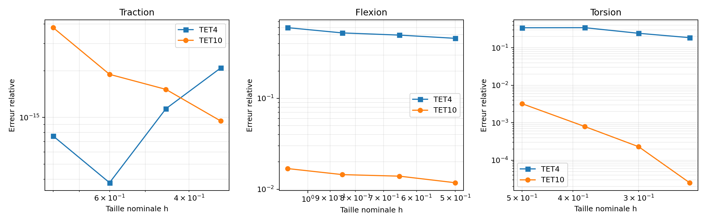 VNV-TET10-STRUCTURAL-CONVERGENCE-012TET10 structural mesh convergenceTET10 bending error: 1.179%Read model, result and limits →
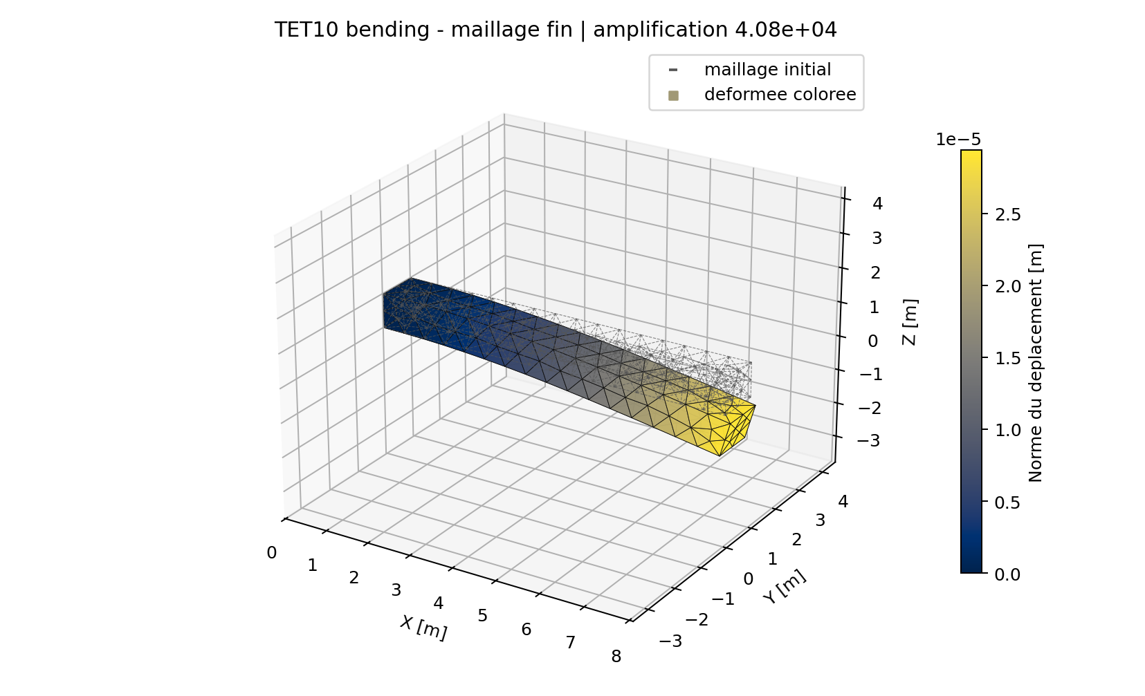 VNV-TET10-STRUCTURAL-CONVERGENCE-012-BTET10 cantilever bending shapeDisplay amplification: 40,800×Read model, result and limits →
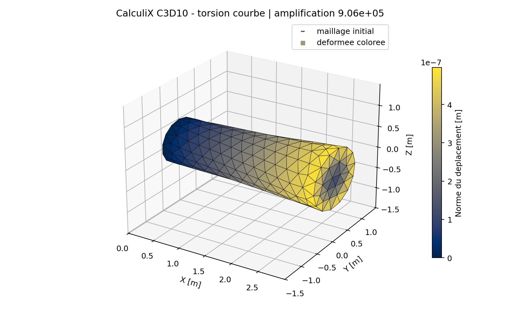 VNV-TET10-CALCULIX-C3D10-014TET10 torsion field correlation with CalculiXRelative full displacement field difference: 6.84 × 10⁻⁵Read model, result and limits →
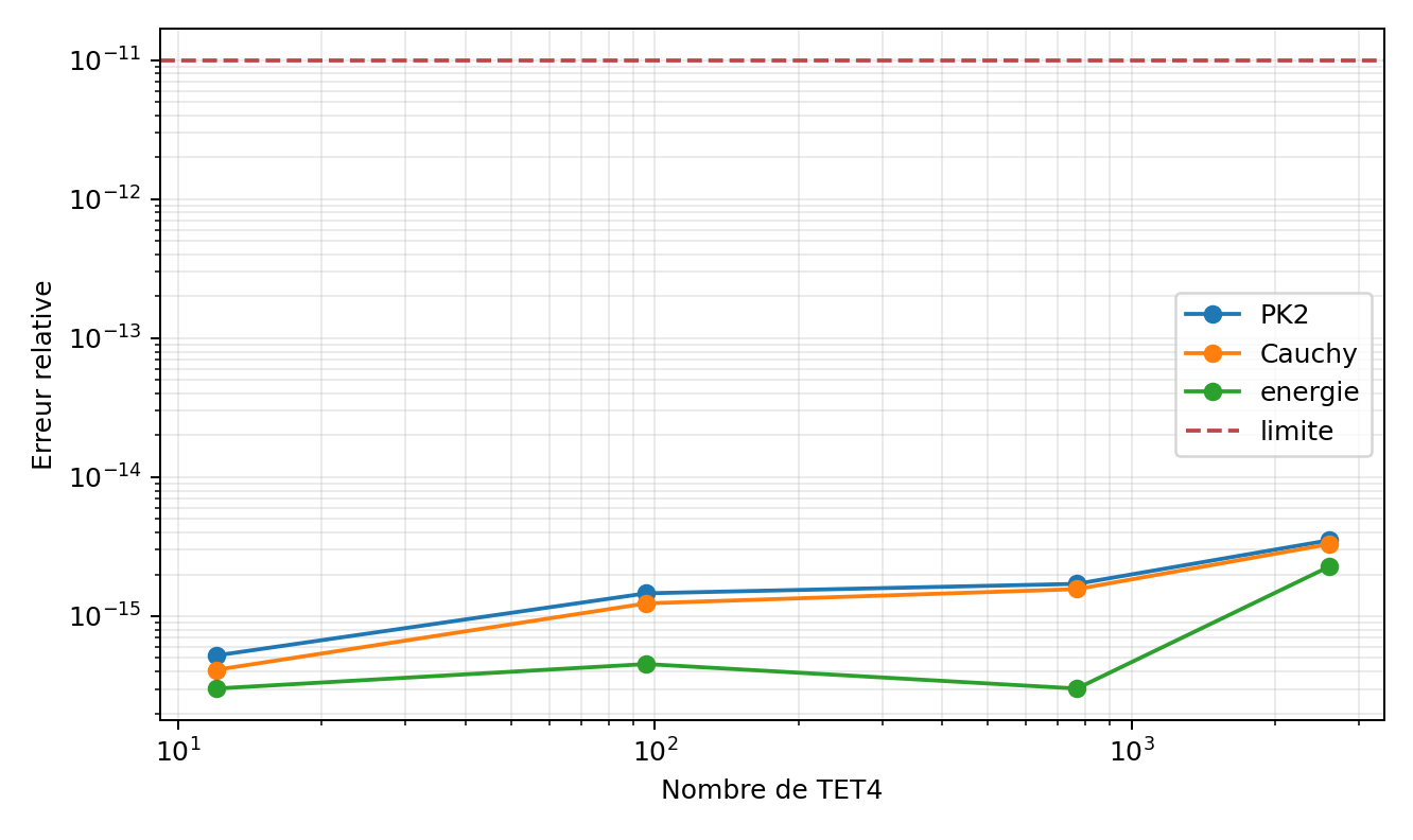 VNV-TET4-TL-STRESS-001TET4 affine finite-strain patchObserved patch error: ≈ 10⁻¹⁵Read model, result and limits →