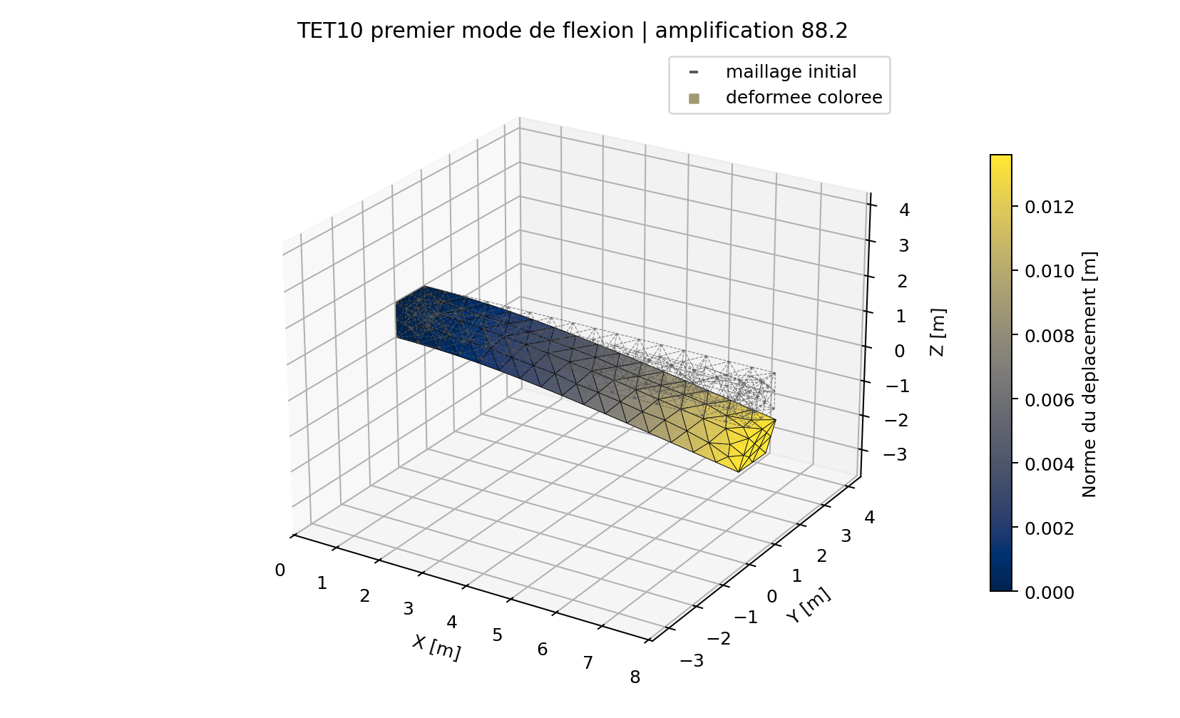
The default sparse path uses eigsh/ARPACK; dense conversion is explicit and bounded by an active-DOF cap.
01 Model and scope
Constrained stiffness and mass define a generalized eigenproblem. Positive eigenvalues map to natural frequencies; eigenvectors are arbitrary up to scale and sign, so residual, mass orthogonality and subspace comparisons matter alongside frequency values.
Route assumptions and calculation checks
- Mass positive-definiteness, residual, mass orthogonality, and effective modal mass are recorded diagnostics.
- Eigenvector sign and scale are arbitrary; repeated modes should be compared as a subspace.
- Shell drilling DOFs without mass may be condensed and reconstructed under a documented route.
Useful foundations and prerequisites
02 Essential equations and symbols
Definitions and conventions
- Stiffness and mass matrices after fixed DOFs and documented massless coordinates are eliminated.
- Eigenvalue equals squared circular natural frequency; λ must be positive for a real oscillation frequency.
- Mode shape: relative displacement pattern, arbitrary in sign and scale until a normalization convention is applied.
- rᵢ
- Dimensionless eigenpair residual; a small value indicates the computed vector satisfies the discrete equation.
- Mass orthogonality for distinct modes under mass normalization; degenerate/repeated eigenspaces need subspace comparisons.
- fᵢ
- Natural frequency in hertz; distinct from angular frequency ω in radians per second.
03 Step by step derivation
Follow the assumptions, equations and discrete operations in order. The full explanation stays visible.
With homogeneous constraints eliminated, free coordinates satisfy M_ff q̈ + K_ff q = 0. Assume harmonic motion q(t)=φe^{iωt}: then (K_ff−ω²M_ff)φ=0. Set λ=ω²; only positive λ gives a real natural frequency f=√λ/(2π). A computed pair is checked with its residual, while mass-normalized distinct modes satisfy ΦᵀM_ffΦ≈I. These checks diagnose numerical quality; they do not prove every material/element/constraint route is qualified.
1 · Reduce to the free dynamic coordinates
After supports and documented massless coordinates are handled, the semi-discrete undamped system has free-coordinate mass and stiffness matrices. Positive-definite mass on the retained subspace is a precondition for interpreting the eigenvalues as ordinary structural frequencies.
2 · Assume harmonic motion
Substitute a sinusoidal mode q(t)=φ exp(iωt). The acceleration contributes −ω²φ, giving the generalized eigenproblem. The solver sets λ=ω²; only positive real λ yields a real undamped natural frequency.
3 · Normalize and compare modes correctly
Mass normalization makes distinct modes orthonormal under M when the matrices are symmetric and the eigenvalues are distinct. The sign and scale of each eigenvector are arbitrary. Nearly repeated modes may rotate within the same eigenspace, so compare subspaces or mass-weighted correlation rather than component signs alone.
4 · Check solver quality and report the route
Record residuals, orthogonality, effective modal mass, mass definiteness, requested mode count, and the selected sparse or bounded dense route. Shell drilling coordinates without physical mass may need documented condensation and reconstruction; that transformation is part of the result's provenance.
04 Algorithm and implementation
Read the linked versioned source for the actual assembly and solver behavior. The derivation above explains the mathematics and is not a verbatim source excerpt.
05 Verification and limitations
ROUTE-DEPENDENT · registry controls each family
TET4 and MITC4 cases expose frequencies, residuals, and mode-shape comparisons.
Each reference supports its own model, observable and analysis route. Read the original contract and limitations before transferring a conclusion.
See this method in a calculation.
Each case keeps its mesh, measured quantities, source record and limitations attached to the result.