Small-strain 3D law in engineering-Voigt order [xx, yy, zz, xy, yz, xz].
01 Model and scope
This is a local, memoryless 3D constitutive law for infinitesimal strain. It maps the symmetric displacement gradient to Cauchy stress and assumes the same response in every direction. The six-component engineering-Voigt convention is part of the model: shear strains are doubled while shear stresses are not.
Route assumptions and calculation checks
- The last three strain components are engineering shears γij=2εij; the corresponding D diagonal entries are μ.
- The v0.2.11 constructor validates E>0 and −1<ν<0.5; near ν=0.5, bulk stiffness grows and displacement elements may lock.
- The 0.2.8 registry remains the cited qualification baseline. Consult its exact element/analysis row; a current package release does not automatically extend that evidence.
Useful foundations and prerequisites
02 Essential equations and symbols
Definitions and conventions
- Infinitesimal strain tensor; rotations are assumed small enough for the linearized strain measure.
- Young modulus and Poisson ratio; accepted by the v0.2.11 constructor when E>0 and −1<ν<0.5.
- First Lamé modulus, shear modulus, and bulk modulus.
- 6×6 constitutive matrix in [xx, yy, zz, xy, yz, xz] order.
- Engineering shear strain; stress entries τij remain tensor shear stresses.
03 Step by step derivation
Follow the assumptions, equations and discrete operations in order. The full explanation stays visible.
The derivation separates kinematics from constitutive response: displacement gives strain, E and ν determine the Lamé moduli, D maps the declared strain vector to stress, and virtual work turns that pointwise law into element forces and stiffness. It does not select an element, integration rule, nonlinear solver, or qualification row.
1 · Kinematics: from displacement to infinitesimal strain
The material law receives strain, not nodal displacement directly. In the small-displacement-gradient model, the symmetric part of ∇u measures extension and shear while its skew part represents infinitesimal rigid rotation. The approximation discards products of displacement gradients; it is not an exact finite-rotation or finite-strain measure.
Rigid translation gives ε=0. In the linearized model, an arbitrarily large rigid rotation is not represented objectively; use a documented finite-kinematic route when that matters.
2 · Isotropy and the volumetric/deviatoric split
An isotropic elastic solid has only two independent moduli. The shear modulus μ controls shape change; the bulk modulus K controls volume change. The Lamé modulus λ couples normal strains in the 3D constitutive matrix. This split exposes why the response becomes numerically difficult near the incompressible limit.
W is strain-energy density per reference/current volume in this infinitesimal linear model. E and ν alone do not describe plasticity, damage, rate effects, or temperature dependence.
3 · Convert the tensor law to the code's Voigt convention
QF Solver orders strain as [εxx, εyy, εzz, γxy, γyz, γxz] and stress as [σxx, σyy, σzz, τxy, τyz, τxz]. The off-diagonal strain entries are engineering shears γij=2εij. Consequently the shear diagonal in D is μ, not 2μ; mixing tensor and engineering shear conventions creates a factor-of-two error.
A uniaxial stress test with free lateral faces should recover εyy=εzz=−νεxx and σxx=Eεxx. That is a useful convention check, not a benchmark for every element route.
4 · Insert the material law into finite-element virtual work
The element interpolation turns nodal coordinates qₑ into strain through ε=Bqₑ. The same constitutive matrix then supplies the internal force and the linear material stiffness. B, geometry mapping, quadrature, and the element family still determine how accurately the element integral is evaluated.
For a homogeneous straight TET4, B and D are constant and Kₑ=VBᵀDB. Higher-order and distorted elements require their own mapped gradients and integration rules.
5 · Material checks, conditioning, and limits
The v0.2.11 material constructor rejects non-positive E and Poisson ratios outside (−1, 0.5). As ν approaches 0.5, K grows without bound in the idealized equations. Standard displacement elements can then lock volumetrically: the computed displacement may be too small even though the constitutive equation is algebraically correct.
These constructor bounds do not qualify a particular element, mesh, analysis, solver, or material/geometry composition. The linked registry controls that claim; near-incompressible behavior needs a formulation and benchmark intended for that regime.
04 Algorithm and implementation
Source excerpt · v0.2.11
The v0.2.11 material constructor checks the admissible constants, then builds the 6×6 stiffness in the documented engineering-shear order.
Functions shown: elasticity_matrix
@cached_property
    def elasticity_matrix(self) -> np.ndarray:
        factor = self.E / ((1.0 + self.nu) * (1.0 - 2.0 * self.nu))
        lam = self.nu * factor
        mu = self.E / (2.0 * (1.0 + self.nu))
        matrix = np.zeros((6, 6), dtype=float)
        matrix[:3, :3] = lam
        np.fill_diagonal(matrix[:3, :3], lam + 2.0 * mu)
        matrix[3, 3] = matrix[4, 4] = matrix[5, 5] = mu
return matrix05 Verification and limitations
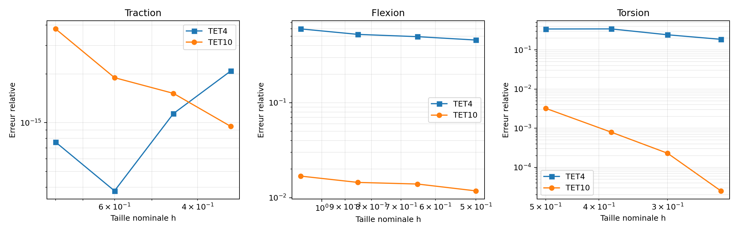
QUALIFIED_BOUNDED · recorded element/analysis combinations only
Each reference supports its own model, observable and analysis route. Read the original contract and limitations before transferring a conclusion.
See this method in a calculation.
Each case keeps its mesh, measured quantities, source record and limitations attached to the result.